Transfer Learning for Bird Species Classification Using Pre-trained Models

In this tutorial, we will explore how to use transfer learning to classify bird species using popular pre-trained models like InceptionV3, VGG16, and InceptionResNetV2. Transfer learning allows us to leverage the knowledge gained from large datasets like ImageNet and apply it to our bird species classification task, saving us time and computational resources.

Why Transfer Learning?

Instead of training a model from scratch, which can be time-consuming and require a large dataset, transfer learning helps by:

1. Utilizing pre-trained models that have already learned relevant features from massive datasets.
2. Fine-tuning these models for specific tasks like classifying bird species.
3. Reducing overfitting when working with smaller datasets by using generalized features.

In this tutorial, we will demonstrate how to load pre-trained models, modify them for our specific classification task, and fine-tune them using a bird species dataset.

Prerequisites

• Basic knowledge of deep learning and Keras.

• Understanding of convolutional neural networks (CNNs) and image classification.

• A dataset of bird species, which should be organized in a folder structure like:

  birds/
    ├── train/
    │   ├── species_1/
    │   ├── species_2/
    └── validation/
        ├── species_1/
        ├── species_2/

Let's begin by loading our dataset and pre-trained models.

Step 1: Extracting the Bird Species Dataset

Before starting our transfer learning task, we need to extract the dataset containing bird species images. The dataset is provided in a .tgz (tar gzip) compressed format, which we will extract using the Python tarfile module.

Explanation

1. Importing the tarfile module: We use Python's tarfile module, which allows us to read and extract files from a .tgz compressed file.
2. Specifying the path to the .tgz file: We define the path to our bird species dataset. In this case, it's stored in the Kaggle input directory.
3. Extracting the first .tgz file: The tarfile.open() function opens the .tgz file in read mode ("r:gz"). The tar.extractall() method then extracts all the contents into the current directory ("./").
4. Extracting the second .tgz file: We repeat the process for a second compressed file, which might contain segmentations or annotations.
5. Confirmation message: After both files are extracted, a message is printed to indicate that the extraction process is complete.

Now that the dataset is ready, we can proceed with loading and preparing it for our transfer learning task.

Step 2: Importing Required Libraries

In this step, we will import several essential libraries that will help us analyze, visualize, and manipulate the bird species dataset.

Explanation:

1. Numpy (np): This library is fundamental for numerical operations in Python. It provides support for arrays and matrices, along with a collection of mathematical functions to operate on these data structures.

2. Pandas (pd): Pandas is a powerful data manipulation and analysis library. It offers data structures like DataFrames that are useful for handling structured data, such as our bird species dataset, which may contain labels and image paths.

3. Matplotlib (plt): Matplotlib is a plotting library used for creating static, interactive, and animated visualizations in Python. We will use it to visualize the data and the results of our model training.

4. Seaborn (sns): Seaborn is built on top of Matplotlib and provides a high-level interface for drawing attractive statistical graphics. It makes it easier to create complex visualizations with less code.

5. Warnings Module: We import the warnings module and use warnings.filterwarnings("ignore") to suppress any warnings that may arise during the execution of our code. This can help keep our output clean and focused on the results we are interested in.

By importing these libraries, we are setting up our environment for effective data manipulation and visualization as we move forward with our analysis and modeling.

Step 3: Exploring the Dataset Structure

Next, we will explore the directory structure of the extracted dataset to better understand how the images are organized.

Explanation:

1. Importing the os module: This module provides a way to use operating system-dependent functionality like reading or writing to the file system.

2. Defining the parent directory path: We specify the path to the parent directory where the images are stored. In this case, it points to the images extracted from our dataset.

3. Listing directories: We use a list comprehension to iterate through the contents of the parent directory with os.listdir(parent_directory). For each item d, we check if it is a directory using os.path.isdir(). This ensures that we only include directories in our list.

4. Sorting the directories: We then sort the list of directories alphabetically using sorted(). This helps us easily navigate through different bird species.

5. Printing the directory names: Finally, we print the sorted list of directories, which represent different bird species in the dataset. Each directory name corresponds to a specific species, containing images associated with that species.

This exploration step helps us understand how to access the images for each species, which will be essential for preparing our data for training the model.

Step 4: Creating Masked Images for Training, Validation, and Testing

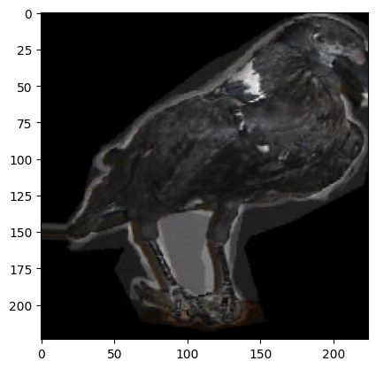
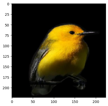
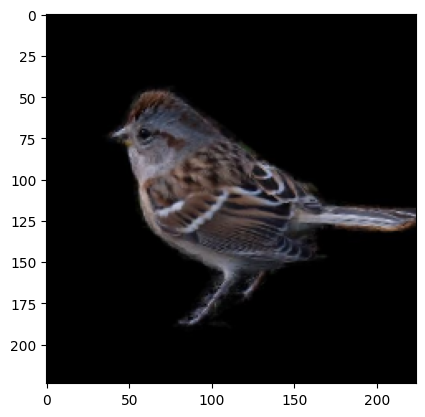
In this step, we will create masked images from the original bird species images and their corresponding segmentation masks. This will help us focus on the relevant parts of the images for our model training.

Explanation:

1. Importing the Image module: We import the Image class from the PIL (Python Imaging Library) module, which allows us to handle and manipulate images easily.

2. Defining the mask_image function: This function takes the list of directories (each representing a bird species) and processes the images within those directories.

3. Creating a directory for masked images: The os.makedirs() function creates a new directory named Masked_Images where we will save our masked images. The exist_ok=True parameter ensures that no error is raised if the directory already exists.

4. Iterating through each species directory: For each directory in directories, we build the path to the images and segmentation masks.

5. Listing image and segmentation files: We gather all JPEG image files and PNG segmentation files from their respective directories. This is done using list comprehensions to filter the files based on their extensions.

6. Shuffling and splitting indexes: We generate an array of indexes corresponding to the images, shuffle them randomly, and then split them into training, validation, and testing sets. This ensures that the data is divided into 80% for training (with 75% of that for training and 25% for validation) and 20% for testing.

7. Loading images and masks: For each set (train, validation, test), we loop through the image and mask pairs. We use Pillow to load the original image and its corresponding segmentation mask, converting the mask to grayscale.

8. Resizing and normalizing the mask: The mask is resized to match the dimensions of the original image, and its pixel values are normalized to the range [0, 1].

9. Applying the mask: We apply the mask to the original image, effectively highlighting the relevant parts.

10. Saving the masked images: The resulting masked image is saved in the Masked_Images directory under the appropriate subdirectory for train, validation, or test sets.

This process is crucial for preparing our data, as it allows the model to focus on the relevant features of the images during training.

Step 5: Data Preprocessing and Augmentation

Now that we have our masked images prepared, we will set up data preprocessing and augmentation techniques to improve the model's robustness and performance.

Explanation:

1. Importing TensorFlow and Keras modules: We import the necessary modules from TensorFlow and Keras, including layers and ImageDataGenerator, which will help us preprocess our image data.

2. Setting constants: We define BS (batch size) as 32 and image_size as (224, 224). This size is compatible with popular transfer learning models such as InceptionV3 and VGG16, which typically accept images of this dimension.

3. Creating data augmentation for the training set: We instantiate the ImageDataGenerator for the training data with various augmentation techniques:

   • rescale=1./255: Normalize pixel values to the range [0, 1].
   • rotation_range=10: Randomly rotate images by up to 10 degrees.
   • width_shift_range=0.1 and height_shift_range=0.1: Randomly shift images horizontally or vertically by up to 10% of their width or height.
   • shear_range=0.1: Apply shearing transformations.
   • zoom_range=0.1: Randomly zoom into images.
   • horizontal_flip=True: Randomly flip images horizontally.
   • fill_mode='nearest': Fill in newly created pixels with the nearest pixel values.

4. Preparing validation and test data generators: For validation and test datasets, we use a simpler ImageDataGenerator that only rescales the images without augmentation.

5. Creating data generators: We use the flow_from_directory method to generate batches of image data from the specified directory structure:

   • Training data: The generator reads images from ./Masked_Images/train, resizes them to image_size, assigns labels as categorical, and specifies the color mode as RGB.
   • Validation data: The generator reads images from ./Masked_Images/valid using the same parameters.
   • Test data: The generator reads images from ./Masked_Images/test using the same parameters.

6. Visualizing training samples: To get a sense of our training data, we visualize a few images from the train_generator. We call next(train_generator) to retrieve the next batch of images and labels, then use plt.imshow() to display the first image in the batch.

This data preprocessing and augmentation setup will enhance the model's ability to generalize by providing it with diverse training samples.

Step 6: Model Definition and Training with VGG16

In this step, we will define our transfer learning model using the VGG16 architecture and train it on our bird species dataset.

Explanation:

1. Importing VGG16: We import the VGG16 model from tensorflow.keras.applications. VGG16 is a well-known convolutional neural network architecture pre-trained on the ImageNet dataset, which allows us to leverage its learned features.

2. Loading the VGG16 model: We instantiate the VGG16 model with the following parameters:

   • input_shape=(224, 224, 3): Specifies the input image size (height, width, channels).
   • include_top=False: Excludes the fully connected output layers (top) of the model, as we will add our own classifier.
   • weights='imagenet': Loads the weights pre-trained on the ImageNet dataset.

3. Freezing the base model: We set vgg16_model.trainable = False to freeze the layers of the VGG16 model. This prevents their weights from being updated during training, allowing us to retain the learned features.

4. Building the Sequential model: We create a new sequential model model_vgg16 and add layers:

   • vgg16_model: The frozen base model.
   • layers.Flatten(): Flattens the output from the base model to a 1D vector.
   • layers.Dense(units=1950, activation='relu'): Adds a fully connected layer with 1950 units and ReLU activation.
   • layers.BatchNormalization(): Applies batch normalization to stabilize and accelerate training.
   • layers.Dense(units=200, activation='softmax'): Adds the final output layer with 200 units (corresponding to the 200 bird species) and softmax activation for multi-class classification.

5. Model summary: We call model_vgg16.summary() to print a summary of the model architecture, showing the layers, output shapes, and the number of parameters.

6. Compiling the model: We compile the model using the following parameters:

   • optimizer='adam': The Adam optimizer for efficient training.
   • loss='categorical_crossentropy': The loss function suitable for multi-class classification.
   • metrics=['accuracy']: We monitor accuracy as a performance metric.

7. Early stopping callback: We set up early stopping using EarlyStopping, which will halt training if the validation loss does not improve for 10 consecutive epochs (patience=10). This helps prevent overfitting.

8. Fitting the model: We train the model using the fit method:

   • train_generator: The training data.
   • validation_data=valid_generator: The validation data for monitoring performance.
   • epochs=100: The maximum number of epochs to train.
   • verbose=1: Display detailed training output.
   • callbacks=[early_stop]: Include the early stopping callback.

Training the model will adjust the weights of the last layers while preserving the learned features of the VGG16 model, effectively fine-tuning it for our specific bird species classification task.

Step 7: Evaluating the Model and Saving It

In this step, we will evaluate the performance of our trained VGG16 model on the test dataset and save the model for future use.

Explanation:

1. Evaluating the Model:
   • We use the evaluate method on model_vgg16 to assess its performance on the test dataset.
   • test_generator provides the test images and their corresponding labels.
   • This function returns the loss value and any additional metrics specified during model compilation, such as accuracy. It allows us to understand how well the model generalizes to unseen data.
2. Saving the Model:
   • We save the trained model to a file named 'bird_CNN_model_vgg16.h5' using the save method. This file contains:
     • The architecture of the model.
     • The weights of the trained model.
     • The training configuration.
   • Saving the model allows you to easily reload it in future sessions for inference or further training without needing to retrain it from scratch.

By evaluating the model, you can determine its effectiveness on the test set, and saving it ensures that you can reuse the trained model later, streamlining the workflow for deploying the model in a production environment or for further experimentation.

Step 8: Building and Training the InceptionResNetV2 Model

In this step, we will create a model using the InceptionResNetV2 architecture, fit it to our training data, and visualize the training and validation accuracy and loss.

Explanation:

1. Loading InceptionResNetV2:
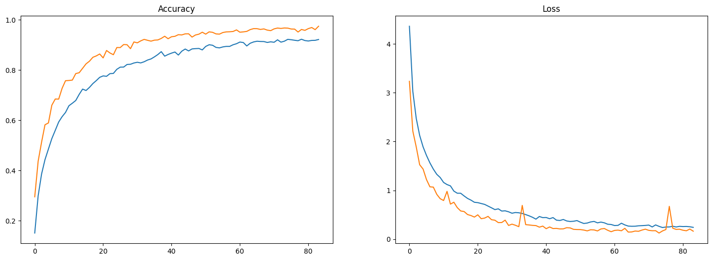
   • We initialize the InceptionResNetV2 model from Keras applications.
   • input_shape=(224, 224, 3) specifies the input dimensions and color channels.
   • include_top=False means we exclude the fully connected layers at the top of the network, allowing us to customize the output layer.
   • weights='imagenet' loads pre-trained weights from ImageNet.
2. Freezing the Base Model:
   • resnet_model.trainable = False freezes the base layers of the model to retain the learned features from the ImageNet dataset. This is crucial for transfer learning, as we want to leverage the pre-trained features without modifying them during the initial training phase.
3. Constructing the Sequential Model:
   • We build a sequential model that consists of:
     • The InceptionResNetV2 model.
     • A flattening layer to convert the 3D outputs to 1D.
     • A dense layer with 1950 units and ReLU activation.
     • A batch normalization layer to stabilize learning.
     • The final output layer with softmax activation for multi-class classification (200 classes, corresponding to bird species).
4. Model Summary:
   • model_resnet.summary() prints the architecture of the model, showing the number of parameters at each layer.
5. Compiling the Model:
   • We compile the model with:
     • optimizer='adam': A popular optimizer that adapts the learning rate during training.
     • loss='categorical_crossentropy': Suitable for multi-class classification problems.
     • metrics=['accuracy']: To monitor accuracy during training and validation.
6. Early Stopping:
   • We implement early stopping to prevent overfitting by monitoring the validation loss. If the validation loss does not improve for 10 consecutive epochs, training will stop.
7. Fitting the Model:
   • The fit method trains the model on the training dataset while validating it on the validation dataset for a maximum of 100 epochs.
   • The verbose=1 parameter shows the progress of training.
8. Creating a DataFrame:
   • We convert the history.history object into a Pandas DataFrame for easier manipulation and visualization of training results.
9. Plotting Accuracy and Loss:
   • We create a figure with two subplots:
     • The first subplot displays the training and validation accuracy over epochs.
     • The second subplot shows the training and validation loss over epochs.
   • This visualization helps us understand how well the model is performing and whether it is overfitting.

Explanation:

1. Model Evaluation:
   • The evaluate method assesses the model's performance on the test dataset using the test generator we defined earlier.
   • This method returns the loss value and metrics specified during compilation (in this case, accuracy).
   • Evaluating on a separate test set helps us understand how well the model generalizes to unseen data, which is crucial for assessing its practical applicability.
2. Saving the Trained Model:
   • The save method saves the entire model architecture, weights, and training configuration to a single HDF5 file (.h5 format).
   • This allows us to easily reload the model later for inference or further training without needing to retrain it from scratch.
   • It's a good practice to save the model after training, especially when the model has shown satisfactory performance on the validation and test datasets.

Step 10: Training the EfficientNetB0 Model

In this step, we will train the EfficientNetB0 model on the bird species dataset. This model is known for its efficiency and accuracy in image classification tasks.

Explanation:

1. Loading EfficientNetB0:
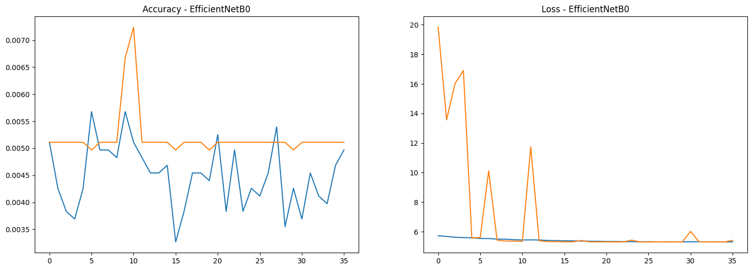
   • We import EfficientNetB0 from Keras applications. This model is pre-trained on ImageNet and is suitable for image classification tasks.
   • The include_top=False argument indicates that we do not want the final classification layer of the model, as we will add our own.
2. Freezing the Model:
   • Setting trainable = False freezes the layers of the pre-trained model, preventing them from being updated during training. This allows us to leverage the learned features while training only the new layers we add.
3. Constructing the Model:
   • We create a Sequential model and add the pre-trained EfficientNetB0 model as the first layer.
   • We then flatten the output from the EfficientNet model to create a single dimension, making it suitable for the dense layers.
   • A dense layer with 1950 units and ReLU activation is added, followed by batch normalization to stabilize the learning process.
   • The final dense layer has 200 units (one for each bird species) with softmax activation to output probabilities for each class.
4. Compiling the Model:
   • The model is compiled with the Adam optimizer, which is efficient for training deep learning models.
   • We use categorical crossentropy as the loss function since this is a multi-class classification problem.
   • Accuracy is chosen as the evaluation metric.
5. Early Stopping:
   • We use EarlyStopping to monitor the validation loss. If the validation loss does not improve for 10 consecutive epochs, training will stop to prevent overfitting.
6. Training the Model:
   • The model is trained on the training dataset and validated on the validation dataset for up to 100 epochs, with real-time updates on the training progress.
7. Visualizing the Training Results:
   • We create a DataFrame from the training history to facilitate the plotting of accuracy and loss.
   • Two subplots are generated: one for accuracy and one for loss, allowing us to visually assess the model's performance over the training epochs.

This concludes the training process for the EfficientNetB0 model on the bird species dataset. You can compare the results of this model with the previously trained VGG16 and InceptionResNetV2 models to determine which performs best.

Step 11: Evaluating the Model and Saving It

After training the EfficientNetB0 model, it's essential to evaluate its performance on a separate test dataset to understand how well it generalizes to unseen data. Additionally, we will save the model so that it can be reused later without needing to retrain.

Explanation:

1. Evaluating Performance:
   • The evaluate method computes the loss and accuracy of the model on the test dataset (from test_generator).
   • The results are printed, showing how well the model performs on the test set.
2. Saving the Model:
   • The save method stores the entire model (architecture, weights, and training configuration) in an HDF5 file (bird_CNN_model_efficientnet.h5).
   • This saved model can be loaded later for inference or further training without starting from scratch.

This step completes the workflow for training and evaluating the EfficientNetB0 model on the bird species dataset.

Step 12: Implementing InceptionV3 Model

Explaination

• Model Architecture:
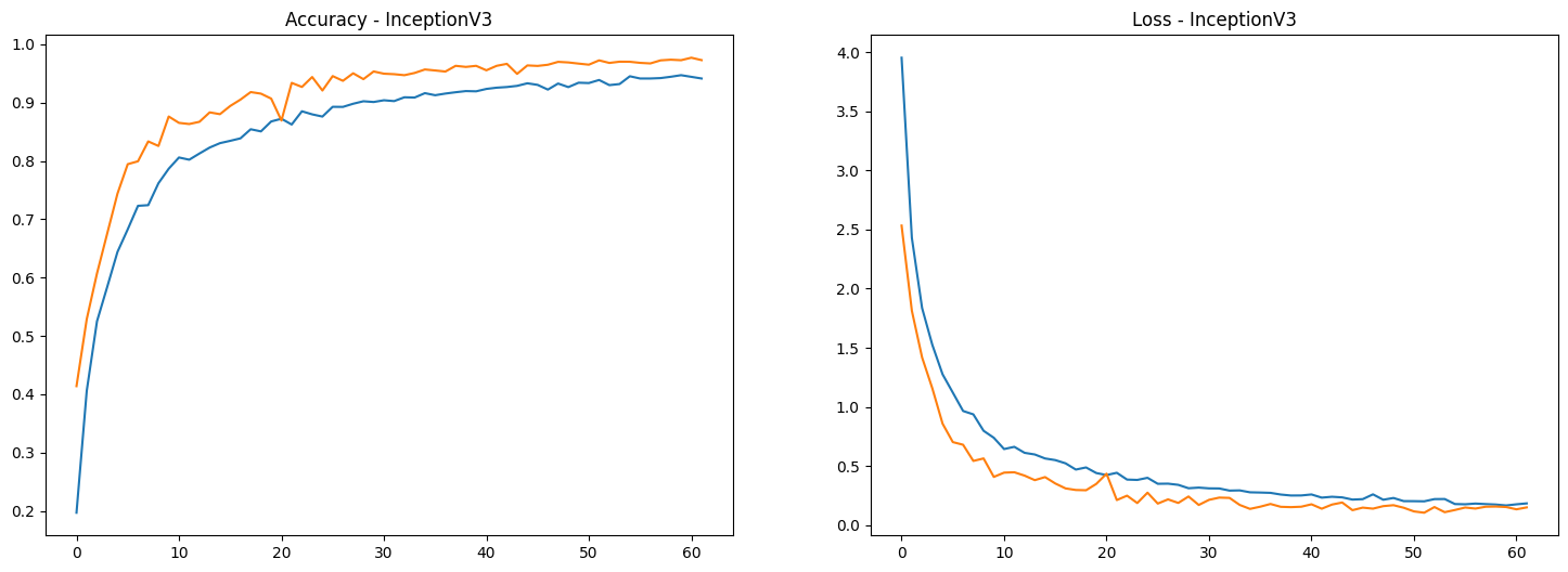
  • The InceptionV3 model is loaded without the top layer (include_top=False) to adapt it to your specific classification task.
  • The model's weights are initialized from the pre-trained ImageNet dataset.
  • The model architecture includes additional layers for classification.
  • The model is compiled with Adam optimizer and categorical crossentropy loss function.
  • The training process includes early stopping to prevent overfitting.
  • The training accuracy and validation accuracy, along with loss values, are plotted for visual analysis of model performance over epochs.

Final Steps: Evaluating and Saving the Model

Explanation:

• Model Evaluation:
  • The evaluate method computes the loss and accuracy of the model on the provided test dataset (test_generator). This gives you an idea of how well your model is likely to perform on unseen data.
• Printing Results:
  • The test loss and accuracy are printed out to the console for quick reference.
• Model Saving:
  • The save method stores the model architecture, weights, and training configuration in an HDF5 file (bird_CNN_model_inceptionv3.h5). This allows you to load the model later without needing to retrain it.

Conclusion

In this tutorial, we explored the process of building a convolutional neural network (CNN) for bird species classification using various pre-trained models, including VGG16, InceptionV3, EfficientNetB0, and InceptionResNetV2. Here’s a summary of what we accomplished:

1. Data Preparation:
   • We extracted the dataset containing images and segmentation masks of different bird species.
   • The data was organized into training, validation, and test sets, ensuring that our model could learn effectively while being evaluated on unseen data.
2. Model Selection and Training:
   • We employed state-of-the-art transfer learning techniques by leveraging pre-trained models, which significantly reduce training time and improve performance.
   • Each model was fine-tuned by adding custom layers for classification tasks and training them on the prepared dataset.
   • Early stopping was implemented to prevent overfitting, ensuring our models maintained good generalization on unseen data.
3. Model Evaluation and Saving:
   • After training, we evaluated the models on a separate test set to gauge their performance, focusing on metrics such as accuracy and loss.
   • Finally, we saved the trained models for future use, allowing for easy deployment in real-world applications or further experimentation.

Key Takeaways:

• Transfer Learning: Using pre-trained models significantly enhances performance and speeds up the training process, especially when working with limited datasets.
• Data Augmentation: Implementing techniques such as rotation, shifting, and flipping helps improve model robustness by exposing it to a wider variety of images.
• Evaluation Metrics: Always evaluate your model on a dedicated test set to ensure it performs well on unseen data.

Next Steps:

• You can further enhance your models by experimenting with additional hyperparameters, exploring more complex architectures, or applying techniques such as fine-tuning on the pre-trained models.
• Consider deploying your trained models using web frameworks or mobile applications to make your bird classification system accessible to users.
• Finally, you can apply the concepts learned in this tutorial to other datasets and domains, expanding your knowledge and skills in deep learning and computer vision.